Multi-armed Bandits

A k-armed Bandit Problem

In our $k$-armed bandit problem, each of the $k$ actions has an expected or mean reward given that that action is selected; let us call this the value of that action. We denote the action selected on time step $t$ as $A_t$, and the corresponding reward as $R_t$. The value then of an arbitrary action $a$, denoted $q_*(a)$, is the expected reward given that a is selected:

$$\begin{gather*} q_*(a) \doteq \mathbb{E}[R_t|A_t=a]. \end{gather*}$$

$q_*(a)$ is not known, so we need to estimate it. We denote the estimated value of action a at time step $t$ as $Q_t(a)$. We would like $Q_t(a)$ to be close to $q_*(a)$.

Sample Average Method

$$\begin{gather*} Q_t(a) \doteq {\text{sum of rewards when a taken prior to t} \over \text{number of times a taken prior to t}} = {\sum_{i=1}^{t-1} R_i \cdot \mathbb{1}_{A_i=a} \over \sum_{i=1}^{t-1} \mathbb{1}_{A_i=a}} \end{gather*}$$

By the law of large numbers, $Q_t(a)$ converges to $q_*(a)$.

Greedy Action

The simplest action selection rule is to select one of the actions with the highest estimated value, that is, one of the greedy actions.

$$\begin{gather*} A_t \doteq \argmax_a{Q_t(a)}. \end{gather*}$$

$\varepsilon$-Greedy Method

Greedy action selection always exploits current knowledge to maximize immediate reward; it spends no time at all sampling apparently inferior actions to see if they might really be better. A simple alternative is to behave greedily most of the time, but every once in a while, say with small probability $\varepsilon$, instead select randomly from among all the actions with equal probability, independently of the action-value estimates.

Incremental Implementaton

The action-value methods we have discussed so far all estimate action values as sample averages of observed rewards. We now turn to the question of how these averages can be computed in a computationally efficient manner, in particular, with constant memory and constant per-time-step computation.

Let $Q_n$ denote the estimate of its action value after it has been selected $n - 1$ times, which we can now write simply as

$$\begin{gather*} Q_n \doteq {R_1 + R_2 + \cdots + R_{n-1} \over n-1}. \end{gather*}$$

Given $Q_n$ and the $n$th reward, $R_n$, the new average of all $n$ rewards can be computed by

$$\begin{align*} Q_{n+1} & = {1\over n}\sum_{i=1}^n R_i \\ & = {1\over n}(R_n + \sum_{i=1}^{n-1} R_i) \\ & = {1\over n}(R_n + (n-1){1\over n-1}\sum_{i=1}^{n-1} R_i) \\ & = {1\over n}(R_n + (n-1)Q_n) \\ & = {1\over n}(R_n + nQ_n - Q_n) \\ & = Q_n + {1\over n}[R_n-Q_n] \end{align*}$$

The general form is

$$\begin{gather*} NewEstimate \leftarrow OldEstimate + StepSize[Target - OldEstimate]. \end{gather*}$$

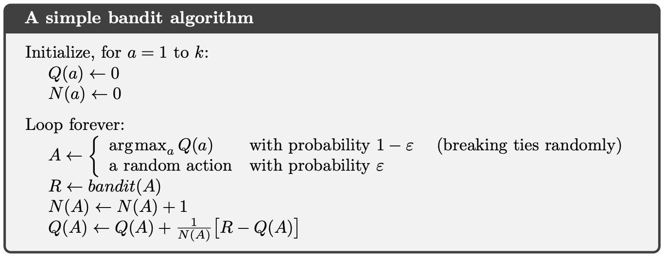
Pseudocode

My Code

Coming soon

Tracking a Nonstationary Problem

As noted earlier, we often encounter reinforcement learning problems that are effectively nonstationary. In such cases, it makes sense to give more weight to recent rewards than to long-past rewards.

$$\begin{align*} Q_{n+1} & \doteq Q_n + \alpha [R_n-Q_n], \alpha \in (0, 1] \\ & = \alpha R_n + (1-\alpha)Q_n \\ & = \alpha R_n + (1-\alpha)[\alpha R_{n-1}+(1-\alpha)Q_{n-1}] \\ & = \alpha R_n + (1-\alpha)\alpha R_{n-1}+(1-\alpha)^2Q_{n-1} \\ & = \alpha R_n + (1-\alpha)\alpha R_{n-1}+(1-\alpha)^2\alpha R_{n-2}+\cdots +(1-\alpha)^{n-1}\alpha R_1+(1-\alpha)^nQ_1 \\ & = (1-\alpha)^nQ_1+\sum_{i=1}^n \alpha(1-\alpha)^{n-i}R_i. \end{align*}$$

The first term tells us that the contribution $Q_1$ decreases exponentially with time. The second term tells us the rewards further back in time contribute exponentially less to the sum. Taken together, we see that the influence of our initialization of $Q$ goes to zero with more and more data. The most recent rewards contribute most to our current estimate.

Optimistic Initial Values

Previously the initial estimated values were assumed to be 0, which is not necessarily optimistic. If we set it to a higher value, by the property of greedy action, the initial reward may not be as big as the initial estimated value. Therefore, it will keep exploring at an early stage.
But, this method is not well-suited for non-stationary problems, and we may not know what the optimistic initial value should be.

Upper-Confidence-Bound (UCB) Action Selection

Exploration is needed because there is always uncertainty about the accuracy of the action-value estimates. It would be better to select among the non-greedy actions according to their potential for actually being optimal, taking into account both how close their estimates are to being maximal and the uncertainties in those estimates. One effective way of doing this is to select actions according to

$$\begin{gather*} A_t \doteq \argmax_a{\biggr [Q_t(a)+c\sqrt{\ln t \over N_t(a)}\biggr ]}, \end{gather*}$$

The idea is that the square-root term is a measure of the uncertainty or variance in the estimate of $a$’s value. The quantity being maxed over is thus a sort of upper bound on the possible true value of action $a$, with $c$ determining the confidence level. Each time $a$ is selected the uncertainty is presumably reduced: $N_t(a)$ increments, and, as it appears in the denominator, the uncertainty term decreases. On the other hand, each time an action other than a is selected, $t$ increases but $N_t(a)$ does not; because t appears in the numerator, the uncertainty estimate increases. The use of the natural logarithm means that the increases get smaller over time, but are unbounded; all actions will eventually be selected, but actions with lower value estimates, or that have already been selected frequently, will be selected with decreasing frequency over time.